The following industrial cases show data of flow production systems that may be found in industry. All data describe existing systems. The data are slightly modified without changing the principal characteristics of the systems.
All systems have been analyzed with the software POM Flowline Optimizer. The analytical results have been compared to simulation results in order to test the precision of the analytical procedures implemented in POM Flowline Optimizer.
System A: Flow line with robots (Production of wheels)
Station |
Buffer size |
Processing time (sec.) |
Availability |
MTTR (sec.) |
[1] - A |
15 |
1 |
1 |
-- |
[2] - B |
1 |
1 |
1 |
-- |
[3] - C |
1 |
9 |
0.99 |
1 |
[4] - D |
20 |
1 |
1 |
-- |
[5] - E |
1 |
12 |
0.99 |
1 |
[6] - F |
1 |
11 |
0.99 |
1 |
[7] - G |
1 |
16 |
0.99 |
1 |
[8] - H |
2 |
16 |
0.99 |
1 |
[9] - I |
4 |
17.125 |
0.99 |
1 |
[10] - J |
5 |
11 |
0.99 |
1 |
[11] - K |
-- |
1 |
0.99 |
1 |
Processing times are deterministic. Some stations are reliable, others are not. Total number of buffers used by the company = 51.
|
# of Buffers |
Analytical |
Simulated |
Deviation |
| Throughput (wheels per sec.) |
51 |
0.05781 |
0.057787 |
0.04% |
The analysis of this system configuration shows that the number of buffer spaces is by far too large. The same throughput as above can be achieved with only 10 buffers that are equally distributed over the system (one buffer space per station).
|
# of Buffers |
Analytical |
Simulated |
Deviation |
| Throughput (wheels per sec.) |
10 |
0.05781 |
0.057791 |
0.03% |
System B: A linear production line with deterministic processing times
This is a small linear system found in the automotive industry.
Station |
Buffer size |
Processing time (sec.) |
Availability |
MTTR (sec.) |
[1] - Stat-1 |
41 |
28.6 |
0.9 |
390 |
[2] - Stat-2 |
50 |
29.1 |
0.9 |
390 |
[3] - Stat-3 |
63 |
29.6 |
0.9 |
390 |
[4] - Stat-4 |
75 |
30 |
0.9 |
390 |
[5] - Stat-5 |
68 |
30 |
0.9 |
390 |
[6] - Stat-6 |
23 |
30 |
0.9 |
390 |
[7] - Stat-7 |
-- |
30 |
0.95 |
300 |
Processing times are deterministic. The stations exhibit failures. Target throughput = 0.0285. The minimum total number of buffers is 320 with the buffer allocation given in the above table.
|
# of Buffers |
Analytical |
Simulated |
Deviation |
| Throughput (wheels per sec.) |
320 |
0.0285 |
0.028035 |
1.64% |
System C: An almost complete automotive body shop (a few stations have been omitted)
This system is a typical automotive manufacturing shop. Processing times are deterministic. Failure data are invented. A few stations of the real system have been omitted.
Station |
Buffer size |
Processing time (sec.) |
Availability |
MTTR (sec.) |
[1] - A0 |
9 |
44 |
0.92 |
240 |
[2] - B0 |
12 |
45 |
0.92 |
240 |
[3] - C0 |
15 |
45 |
0.92 |
240 |
[4] - D0 |
16 |
45 |
0.92 |
240 |
[5] - E0 |
21 |
45.40 |
0.92 |
240 |
[6] - F0 |
21 |
45 |
0.92 |
240 |
[7] - G0 |
19 |
44.9 |
0.92 |
240 |
[8] - H0 |
-- |
46.9 |
0.92 |
240 |
[9] - I0 |
3 |
44.6 |
0.92 |
240 |
[10] - J0 |
3 |
44.6 |
0.92 |
240 |
[11] - K0 |
6 |
44.6 |
0.92 |
240 |
[12] - L0 |
6 |
45 |
0.92 |
240 |
[13] - M0 |
6 |
44.6 |
0.92 |
240 |
[14] - N0 |
9 |
45 |
0.92 |
240 |
[15] - O0 |
9 |
45 |
0.92 |
240 |
[16] - P0 |
9 |
45 |
0.92 |
240 |
[17] - Q0 |
9 |
45 |
0.92 |
240 |
[18] - R0 |
14 |
43 |
0.92 |
240 |
[19] - S0 |
5 |
45.40 |
0.92 |
240 |
[20] - T0 |
4 |
43 |
0.92 |
240 |
[21] - U0 |
14 |
43 |
0.92 |
240 |
[22] - V0 |
4 |
43 |
0.92 |
240 |
[23] - V0 |
5 |
45.40 |
0.92 |
240 |
[24] - X0 |
8 |
43 |
0.92 |
240 |
[25] - Y0 |
9 |
45.40 |
0.92 |
240 |
[26] - Z |
9 |
46 |
0.92 |
240 |
[27] - A1 |
9 |
45.1 |
0.92 |
240 |
[28] - B1 |
9 |
46.4 |
0.92 |
240 |
[29] - C1 |
9 |
46.4 |
0.92 |
240 |
[30] - D1 |
9 |
46.4 |
0.92 |
240 |
[31] - E1 |
8 |
45.90 |
0.92 |
240 |
The following picture shows the layout:
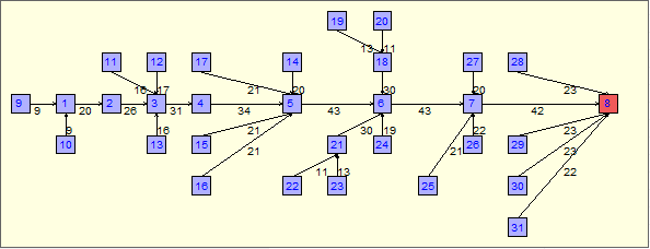
Processing times are deterministic. Target throughput = 0.017 (cars per sec.). The minimum total number of buffers required for this throughput is 289. The detailed allocation of the buffer spaces to the stations is given in the above table.
|
# of Buffers |
Analytical |
Simulated |
Deviation |
| Throughput (cars per sec.) |
289 |
0.017 |
0.01677 |
1.34% |
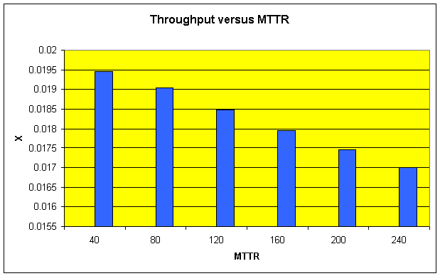
Usually the planners have only limited information about the MTTR-values. Therefore a planner may want to perform a sensitivity analysis in order to see what happens if the assumptions about the MTTR-values are changed. The following table shows the buffer distribution and the throughput for different values of MTTR (assumed equal for all stations). In each case, when the MTTR was changed, the resulting buffer allocation problem (dual problem) for the given total number of buffers was solved. With POM Flowline Optimizer, which implements performance analysis algorithms as well as buffer optimization methods, each buffer optimization required a few seconds.
The table shows that with changing MTTR the buffers are reallocated among the stations. It also shows that for each MTTR a unique optimal buffer distribution results. Thus, in a typical planning process, when the planners perform a sensitivity analysis w.r.t. the failure characteristics of the stations, for each considered system alternative the resulting optimum buffer allocation must be computed.
|
MTTR |
Station |
40 |
80 |
120 |
160 |
200 |
240 |
[1] - A0 |
8 |
8 |
8 |
9 |
8 |
9 |
[2] - B0 |
11 |
11 |
11 |
11 |
11 |
12 |
[3] - C0 |
14 |
14 |
14 |
14 |
14 |
15 |
[4] - D0 |
15 |
15 |
15 |
15 |
15 |
16 |
[5] - E0 |
20 |
19 |
19 |
19 |
20 |
21 |
[6] - F0 |
20 |
19 |
18 |
18 |
19 |
21 |
[7] - G0 |
18 |
17 |
16 |
15 |
15 |
19 |
[8] - H0 |
-- |
-- |
-- |
-- |
-- |
-- |
[9] - I0 |
2 |
4 |
4 |
4 |
3 |
3 |
[10] - J0 |
2 |
4 |
4 |
4 |
3 |
3 |
[11] - K0 |
5 |
6 |
6 |
7 |
7 |
6 |
[12] - L0 |
5 |
6 |
7 |
7 |
7 |
6 |
[13] - M0 |
5 |
6 |
7 |
7 |
7 |
6 |
[14] - N0 |
8 |
8 |
8 |
9 |
9 |
9 |
[15] - O0 |
8 |
8 |
8 |
9 |
9 |
9 |
[16] - P0 |
8 |
8 |
8 |
9 |
9 |
9 |
[17] - Q0 |
8 |
8 |
8 |
9 |
9 |
9 |
[18] - R0 |
13 |
13 |
13 |
13 |
14 |
14 |
[19] - S0 |
4 |
4 |
5 |
6 |
6 |
5 |
[20] - T0 |
3 |
3 |
4 |
4 |
4 |
4 |
[21] - U0 |
13 |
13 |
13 |
13 |
14 |
14 |
[22] - V0 |
3 |
3 |
4 |
4 |
4 |
4 |
[23] - V0 |
4 |
4 |
5 |
5 |
6 |
5 |
[24] - X0 |
7 |
7 |
7 |
8 |
8 |
8 |
[25] - Y0 |
8 |
8 |
8 |
8 |
9 |
9 |
[26] - Z |
8 |
8 |
8 |
8 |
9 |
9 |
[27] - A1 |
8 |
8 |
8 |
8 |
8 |
9 |
[28] - B1 |
15 |
14 |
13 |
11 |
10 |
9 |
[29] - C1 |
16 |
15 |
14 |
12 |
11 |
9 |
[30] - D1 |
16 |
15 |
14 |
12 |
11 |
9 |
[31] - E1 |
14 |
13 |
12 |
11 |
10 |
8 |
Total |
289 |
289 |
289 |
289 |
289 |
289 |
X |
0.019464 |
0.019042 |
0.018479 |
0.017952 |
0.017449 |
0.017 |
The following graph illustrates the influence of the MTTR-values on the throughput.
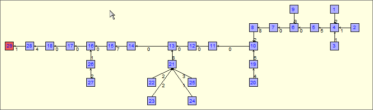
System D: A subsystem of an automotive body shop
This is a subsystem of an automotive body shop where the planner has fixed many buffer sizes to zero due to technical reasons.
Station |
Buffer size |
Processing time (sec.) |
Availability |
MTTR (sec.) |
[1] - A0 |
2 |
128 |
0.961 |
360 |
[2] - A1 |
1 |
128 |
0.982 |
360 |
[3] - A2 |
1 |
128 |
0.982 |
360 |
[4] - A3 |
5 |
128 |
0.961 |
360 |
[5] - A4 |
0 |
128 |
0.9825 |
360 |
[6] - A5 |
0 |
128 |
0.9807 |
360 |
[7] - A6 |
8 |
128 |
0.9944 |
360 |
[8] - A7 |
2 |
60 |
0.998 |
360 |
[9] - A8 |
3 |
128 |
0.9514 |
360 |
[10] - A9 |
0 |
128 |
0.9742 |
360 |
[11] - A10 |
0 |
128 |
0.9912 |
360 |
[12] - A11 |
0 |
128 |
0.9997 |
360 |
[13] - A12 |
0 |
128 |
0.9944 |
360 |
[14] - A13 |
7 |
128 |
0.9924 |
360 |
[15] - A14 |
0 |
128 |
0.9904 |
360 |
[16] - A15 |
0 |
128 |
0.9713 |
360 |
[17] - A16 |
0 |
128 |
0.9912 |
360 |
[18] - A17 |
4 |
128 |
0.995 |
360 |
[19] - A18 |
6 |
128 |
0.974 |
360 |
[20] - A19 |
4 |
128 |
0.9581 |
360 |
[21] - A20 |
8 |
128 |
0.9469 |
360 |
[22] - A21 |
2 |
128 |
0.9869 |
360 |
[23] - A22 |
2 |
128 |
0.9869 |
360 |
[24] - A23 |
1 |
128 |
0.997 |
360 |
[25] - A24 |
3 |
128 |
0.9593 |
360 |
[26] - A25 |
1 |
128 |
0.9791 |
360 |
[27] - A26 |
2 |
128 |
0.9854 |
360 |
[28] - A27 |
1 |
128 |
0.9627 |
360 |
[29] - A28 |
-- |
128 |
0.984 |
360 |
The following picture shows the layout:
|
# of Buffers |
Analytical |
Simulated |
Deviation |
| Throughput (parts per sec.) |
63 |
0.006809 |
0.006759 |
0.73% |
System E: A flow line with manual workstations
The following system is a flow line with manual workstations. The processing times are generally distributed with given mean $\mu$ and given coefficient of variation ($CV=\frac{\sigma}{\mu}$).
Station |
Buffer size |
Processing time (sec.) |
CV(Processing time) |
[1] - Station1 |
-- |
1.87 |
0.5 |
[2] - Station2 |
10 |
1.85 |
0.5 |
[3] - Station3 |
8 |
1.8 |
0.5 |
[4] - Station4 |
8 |
1.72 |
0.5 |
[5] - Station5 |
9 |
1.87 |
0.5 |
[6] - Station6 |
16 |
1.88 |
0.5 |
[7] - Station7 |
17 |
1.88 |
0.5 |
[8] - Station8 |
10 |
1.76 |
0.5 |
[9] - Station9 |
5 |
1.8 |
0.5 |
The results are as follows:
|
# of Buffers |
Analytical |
Simulated |
Deviation |
| Throughput (parts per sec.) |
83 |
0.52 |
0.51795 |
0.39% |
|