The role of the waiting time distribution in a multi-level inventory system
In the following we consider a two-level supply-chain, which is known in the literature as the One-Warehouse-N-Retailer system. Such a system can be found very often in industrial practice. We will show, that the probability distribution of the waiting time of a retailer order at the warehouse has a significant influence on the inventory that is required at the retailer level.
In the example, we make the following assumptions:
- a single warehouse
- using an $(r,s,q)$ inventory policy in discrete time with $r=1$
- deterministic replenishment lead time $L=10$
- holding costs $h=0.024$
- fixed ordering costs $s=120$
- replenishment order size is fixed $q=1000$
- daily review
- 10 identical retailers
- with normally-distributed period (daily) demands ($\mu_D=20$, $\sigma_D=5$)
- using a basestock policy with daily review $(1,S)$
- with holding costs $h=0.024$
- with target service level $\beta=0.9
The following table has been constructed by varying the reorder point in the warehouse $s$. For each reorder point the resulting probability distribution has been computed analytically. With this given probability distribution (which is the replenishment lead time distribution seen by a retailer) for each retailer the optimum basestock level w.r.t. to the target $\beta$ service-level is computed. Finally the average costs on both stages of the supply chain are calculated.
reorder point $s$ |
-200 |
0 |
200 |
400 |
600 |
800 |
900 |
1000 |
1050 |
1100 |
Waiting time
|
$P\{W=w\}$ |
$P\{W=w\}$ |
$P\{W=w\}$ |
$P\{W=w\}$ |
$P\{W=w\}$ |
$P\{W=w\}$ |
$P\{W=w\}$ |
$P\{W=w\}$ |
$P\{W=w\}$ |
$P\{W=w\}$ |
0
|
0 |
0.0032 |
0.1494 |
0.3494 |
0.5494 |
0.7494 |
0.8494 |
0.9462 |
0.9812 |
0.9966 |
1
|
0 |
0.0492 |
0.1 |
0.1 |
0.1 |
0.1 |
0.0971 |
0.0508 |
0.0186 |
0.0034 |
2
|
0.0026 |
0.0969 |
0.1 |
0.1 |
0.1 |
0.0974 |
0.0508 |
|||
3
|
0.0492 |
0.1 |
0.1 |
0.1 |
0.1 |
0.0508 |
||||
4
|
0.0975 |
0.1 |
0.1 |
0.1 |
0.0979 |
|||||
5
|
0.1 |
0.1 |
0.1 |
0.1 |
0.0508 |
|||||
6
|
0.1 |
0.1 |
0.1 |
0.0985 |
||||||
7
|
0.1 |
0.1 |
0.1 |
0.0508 |
||||||
8
|
0.1 |
0.1 |
0.099 |
|||||||
9
|
0.1 |
0.1 |
0.0508 |
|||||||
10
|
0.1 |
0.0994 |
||||||||
11
|
0.1012 |
0.0506 |
||||||||
12
|
0.0992 |
|||||||||
13
|
0.0492 |
|||||||||
warehouse inventory |
0 |
0 |
5.69 |
45.68 |
125.69 |
245.68 |
320.69 |
405.69 |
451.91 |
500.34 |
warehouse costs |
0 |
0 |
0.14 |
1.1 |
3.02 |
5.9 |
7.7 |
9.74 |
10.85 |
12.01 |
expected leadtime |
8.99 |
6.99 |
5.05 |
3.45 |
2.24 |
1.44 |
1.2 |
1.05 |
1.02 |
1 |
basestock level $S$ |
287 |
246 |
205 |
165 |
123 |
83 |
63 |
48 |
45 |
45 |
retailer inventory |
882.52 |
873.67 |
852 |
765.73 |
590.76 |
350.34 |
193.47 |
80.17 |
56.73 |
57.19 |
retailer costs |
21.18 |
20.97 |
20.45 |
18.38 |
14.18 |
8.41 |
4.64 |
1.92 |
1.36 |
1.37 |
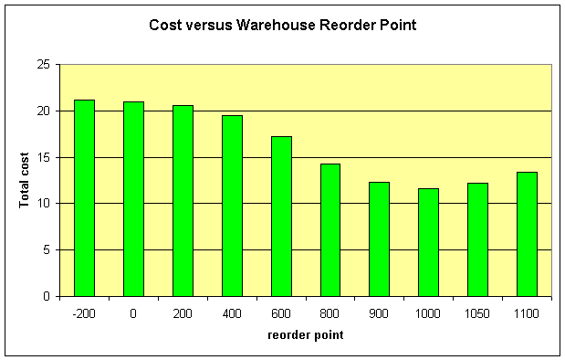
total costs |
21.18 |
20.97 |
20.58 |
19.47 |
17.19 |
14.3 |
12.34 |
11.66 |
12.21 |
13.38 |
Note that the minimum lead time is one period, caused by the discrete review. The results show that in the current setting it is optimal to use a warehouse reorder point $s=1000$ and a retailer basestock level $S=48$. The development of the total cost curve is shown in the following graph.
The procedure used to evaluate the performance of an $(r,s,q)$ policy which is the basis for finding the optimum distribution of the inventory over all nodes in the supply chain is applicable without any change to the case of non-identical retailers. Being able to compute the complete waiting time distribution is the key for the solution of the problem. The remaining calculations are more or less standard.
Further information are available in the book.