7.2 Exponentielle Gl¨attung zweiter Ordnung
Exponentielle Gl¨attung zweiter Ordnung I
y
k
= β
0
+ β
1
·k + ǫ
k
k = t − n + 1, . . . , t
y
(1)
t
= α · y
t
+ (1 − α) · y
(1)
t−1
t = 1, 2, . . .
Exponentielle Gl¨attung zweiter Ordnung II
E
n
y
(1)
t
o
= E {y
t
} − b
1
·
1 − α
α
t = 1, 2, . . .
y
(2)
t
= α · y
(1)
t
+ (1 − α) · y
(2)
t−1
t = 1, 2, ...
E
n
y
(2)
t
o
= E
n
y
(1)
t
o
− b
1
·
1 − α
α
t = 1, 2, ...
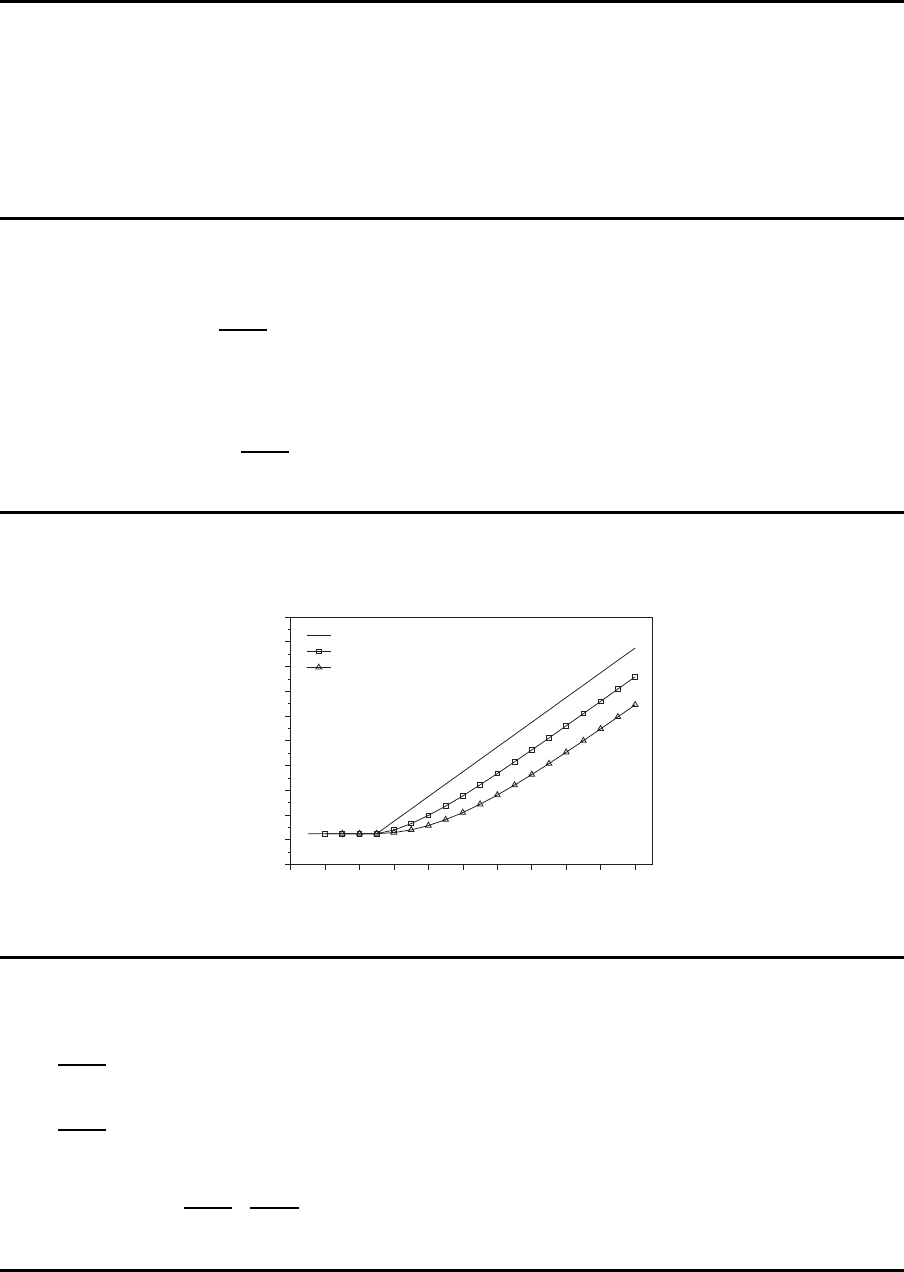
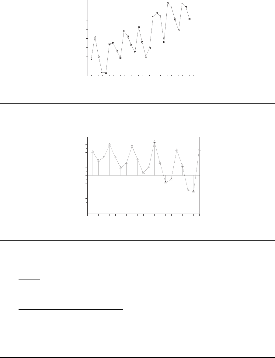
Exponentielle Gl¨attung zweiter Ordnung III
0
4
8
12
16
20
24
28
32
36
40
Bedarfsmenge
0 2 4 6 8 10 12 14 16 18 20
Zeit
t
Beobachtungswerte
Mittelwerte 1. Ordnung
Mittelwerte 2. Ordnung
Exponentielle Gl¨attung zweiter Ordnung IV
b
1,t
=
α
1 − α
·
h
E
n
y
(1)
t
o
− E
n
y
(2)
t
oi
t = 1, 2, ...
b
1,t
=
α
1 − α
·
h
y
(1)
t
− y
(2)
t
i
t = 1, 2, ...
E{y
t
} = E
n
y
(1)
t
o
+
1 − α
α
·
α
1 − α
·
h
E
n
y
(1)
t
o
− E
n
y
(2)
t
oi
17
Exponentielle Gl¨attung zweiter Ordnung V
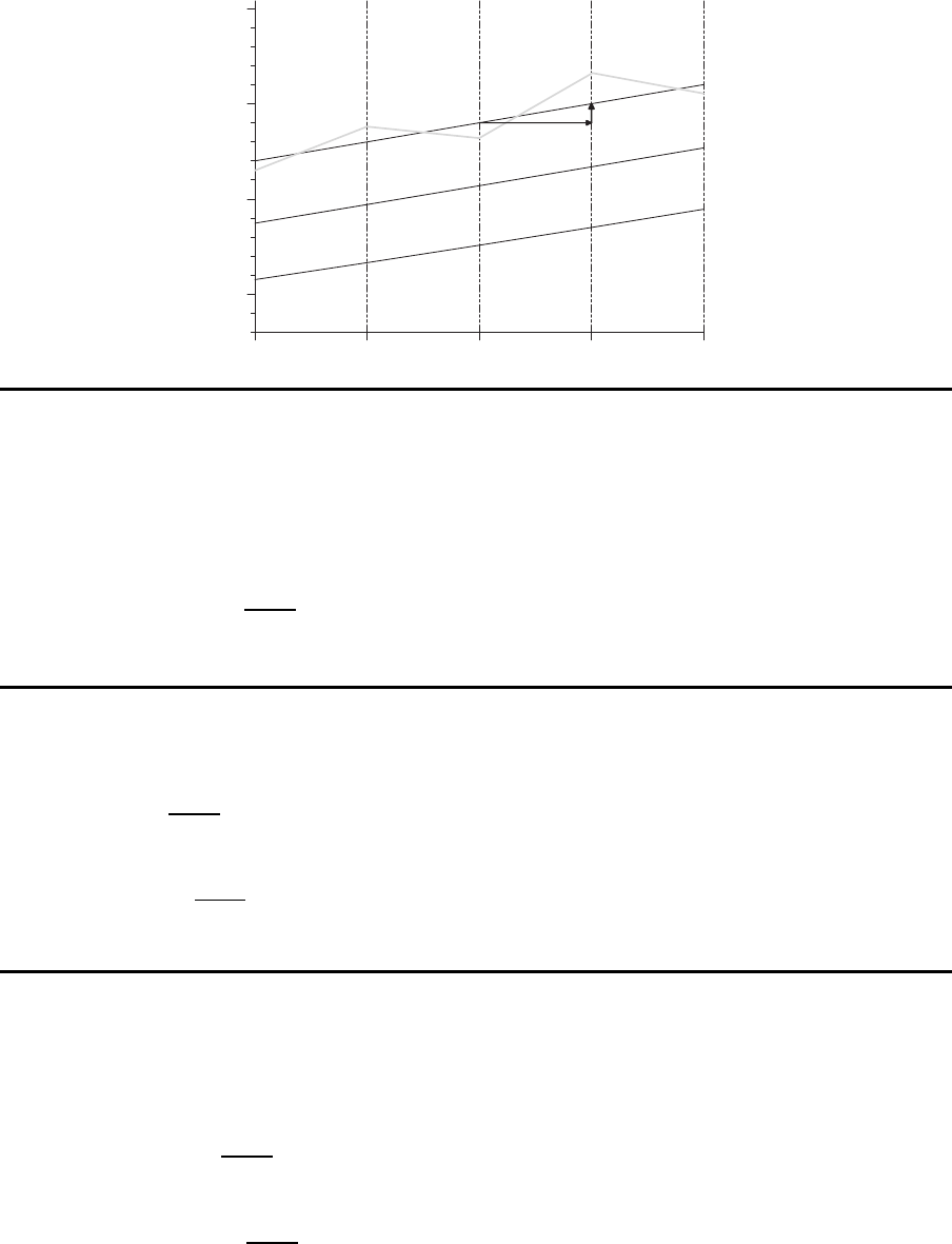
A
B
C
D
t
Beobachtungswerte
Mittelwerte 1. Ordnung
Mittelwerte 2. Ordnung
Trendgerade
t+1
Steigung
Exponentielle Gl¨attung zweiter Ordnung VI
b
0,t
= 2 · y
(1)
t
− y
(2)
t
t = 1, 2, . . .
p
t+j
=
h
2 ·y
(1)
t
− y
(2)
t
i
+
α
1 − α
·
y
(1)
t
− y
(2)
t
·j t = 1, 2, . . .
Exponentielle Gl¨attung zweiter Ordnung VII
y
(1)
0
= b
0,0
− b
1,0
·
1 − α
α
y
(2)
0
= b
0,0
− 2 ·b
1,0
·
1 − α
α
Das Prognoseverfahren
• Start:
Bestimme Startwerte f¨ur die gleitenden Durchschnitte:
y
(1)
0
= b
0,0
− b
1,0
·
1 − α
α
y
(2)
0
= b
0,0
− 2 · b
1,0
·
1 − α
α
Berechne den Prognosewert f¨ur Periode 1:
p
1
= b
0,0
+ b
1,0
18
• Schritt t:
y
(1)
t
= α · y
t
+ (1 − α) · y
(1)
t−1
y
(2)
t
= α · y
(1)
t
+ (1 − α) · y
(2)
t−1
p
t+j
=
h
2 · y
(1)
t
− y
(2)
t
i
+
α
1 − α
·
y
(1)
t
− y
(2)
t
· j
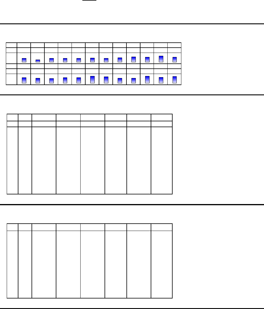
Beispiel
t 1 2 3 4 5 6 7 8 9 10 11 12
y
t
317 194 312 316 322 334 317 356 428 411 494 412
t 13 14 15 16 17 18 19 20 21 22 23 24
y
t
460 395 392 447 452 571 517 397 410 579 473 558
Ergebnisse I
t y
t
y
(1)
t
y
(2)
t
b
0,t
b
1,t
p
t+1
e
t
0 177.0800 79.1600 275.0000 10.8800 285.8800
1 317 191.0720 90.3512 291.7928 11.1912 302.9840 31.12
2 194 191.3648 100.4526 282.2770 10.1014 292.3784 -108.98
3 312 203.4283 110.7502 296.1064 10.2976 306.4040 19.62
4 316 214.6855 121.1437 308.2273 10.3935 318.6208 9.59
5 322 225.4169 131.5710 319.2628 10.4273 329.6902 3.37
6 334 236.2752 142.0414 330.5090 10.4704 340.9794 4.30
7 317 244.3477 152.2720 336.4233 10.2306 346.6539 -23.97
8 356 255.5129 162.5961 348.4297 10.3241 358.7538 9.34
9 428 272.7616 173.6127 371.9105 11.0166 382.9271 69.24
10 411 286.5854 184.9099 388.2609 11.2973 399.5 582 28.07
11 494 307.3269 197.1516 417.5021 12.2417 429.7 438 94.44
12 412 317.7942 209.2159 426.3725 12.0643 438.4 368 -17.74
Ergebnisse II
t y
t
y
(1)
t
y
(2)
t
b
0,t
b
1,t
p
t+1
e
t
13 460 332.0148 221.4958 442.5338 12.2799 454.8 137 21.56
14 395 338.3133 233.1775 443.4491 11.6818 455.1 309 -59.81
15 392 343.6820 244.2280 443.1360 11.0504 454.1 864 -63.13
16 447 354.0138 255.2065 452.8210 10.9786 463.7 996 -7.18
17 452 363.8124 266.0671 461.5577 10.8606 472.4 183 -11.79
18 571 384.5312 277.9135 491.1488 11.8464 502.9 952 98.58
19 517 397.7780 289.9000 505.6561 11.9865 517.6 426 14.00
20 397 397.7003 300.6800 494.7205 10.7800 505.5 005 -120.64
21 410 398.9302 310.5050 487.3554 9.8250 497.1804 -95.50
22 579 416.9372 321.1482 512.7261 10.6432 523.3 693 81.81
23 473 422.5434 331.2877 513.7991 10.1395 523.9 387 -50.36
24 558 436.0891 341.7679 530.4103 10.4801 540.8 904 34.06
19
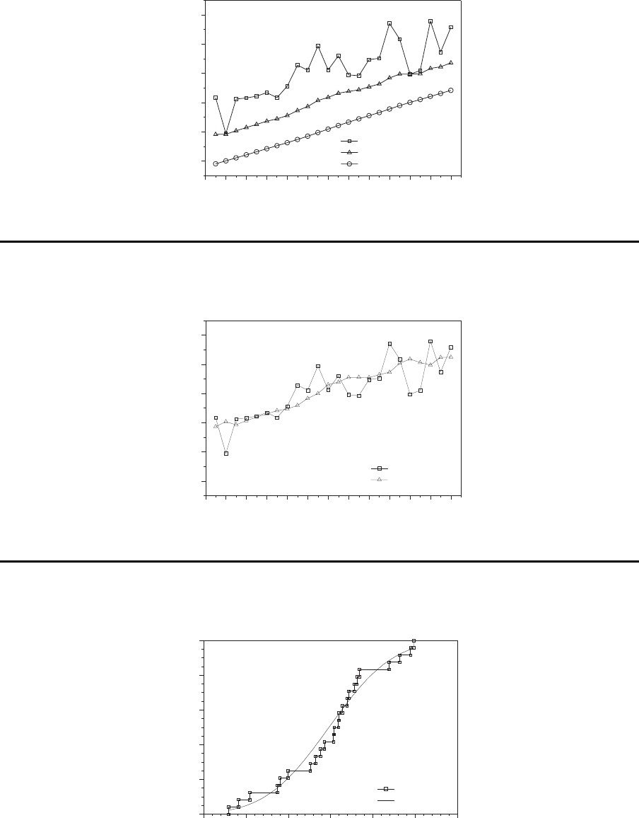
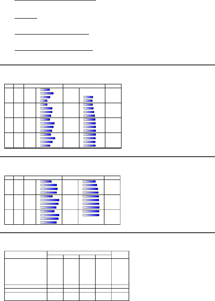
Zeitreihenverl¨aufe
100
200
300
400
500
600
Bedarfsmenge
0 2 4 6 8 10 12 14 16 18 20 22 24
Zeit
t
Beobachtung
Durchschnitt 1. Ordnung
Durchschnitt 2. Ordnung
Prognose
100
200
300
400
500
600
Bedarfsmenge
0 2 4 6 8 10 12 14 16 18 20 22 24
Zeit
t
Beobachtung
Prognose
Prognosefehler
0.0
0.2
0.4
0.6
0.8
1.0
P{e
t
≤
x}
-150 -100 -50 0 50 100 150
Prognosefehler
x
beobachtet
theoretisch
20

7.3 Verfahren von Holt
Verfahren von Holt
Zwei Gl¨attungsparameter
Achsenabschnitt
b
0,t
= α · y
t
+ (1 − α) · (b
0,t−1
+ b
1,t−1
) t = 1, 2, ...
Steigung
b
1,t
= β · (b
0,t
− b
0,t−1
) + (1 − β) · b
1,t−1
t = 1, 2, ...
8 Prognose bei saisonalem Bedarf
8.1 Zeitreihendekomposit ion
Saisonberei nigung
Y
saisonbereinigt
=
Y
S
= T · C · I
Zeitreihendekompo sition I
S · I =
T · C · S · I
T · C
s
m
=
1
n
·
n
X
t=1
si
tm
m = 1, 2, ..., z
Zeitreihendekompo sition II
Quartal m
Jahr t 1 2 3 4 Summe
1 289 410 301 213 1213
2 212 371 374 333 1290
3 293 441 411 363 1508
4 324 462 379 301 1466
5 347 520 540 521 1928
6 381 594 573 504 2052
7 444 592 571 507 2114
21
Zeitreihe
200
250
300
350
400
450
500
550
600
Bedarfsmenge
0 2 4 6 8 10 12 14 16 18 20 22 24 26 28 30
Zeit
(Quartale)
Autokorrelationsfunktion
-0.8
-0.6
-0.4
-0.2
0.0
0.2
0.4
0.6
0.8
1.0
ρ
τ
0.0
0.2
0.4
0.6
0.8
1.0
0 1 2 3 4 5 6 7 8 9 10 11 12 13 14 15 16 17 18 19 20
Zeitverschiebung
τ
Zentrierter gleitender Durchschnitt I
y
(1)
t
=
1
2 · k + 1
·
t+k
X
j=t−k
y
j
y
(2)
t
=
0.5 · y
t−2
+ y
t−1
+ y
t
+ y
t+1
+ 0.5 · y
t+2
4
t = 3, 4, ..., n −2
y
(2)
t
=
y
(1)
t
+ y
(1)
t+1
2
t = 3, 4, ..., n −2
22
Zentrierter gleitender Durchschnitt II
y
(2)
t
=
0.5 · y
t−2
+ y
t−1
+ y
t
+ y
t+1
+ 0.5 · y
t+2
4
t = 3, 4, ..., n −2
y
(2)
t
=
y
(1)
t
+ y
(1)
t+1
2
t = 3, 4, ..., n −2
tc
13
=
0.5 · y
11
+ y
12
+ y
13
+ y
14
+ 0.5 · y
21
4
=
0.5 · 289 + 410 + 301 + 213 + 0.5 · 212
4
= 293.63
TC und SI, Teil 1
t m y
tm
tc
tm
si
tm
1 1 289 – –
1 2 410 – –
1 3 301 293.63 1.0251
1 4 213 279.13 0.7631
2 1 212 283.38 0.7481
2 2 371 307.50 1.2065
2 3 374 332.63 1.1244
2 4 333 351.50 0.9474
3 1 293 364.88 0.8030
3 2 441 373.25 1.1815
3 3 411 380.88 1.0791
3 4 363 387.38 0.9371
4 1 324 386.00 0.8394
4 2 462 374.25 1.2345
4 3 379 369.38 1.0261
4 4 301 379.50 0.7931
TC und SI, Teil 2
t m y
tm
tc
tm
si
tm
5 1 347 406.88 0.8528
5 2 520 454.50 1.1441
5 3 540 486.25 1.1105
5 4 521 499.75 1.0425
6 1 381 513.13 0.7425
6 2 594 515.13 1.1531
6 3 573 520.88 1.1001
6 4 504 528.50 0.9536
7 1 444 528.00 0.8409
7 2 592 528.13 1.1209
7 3 571 – –
7 4 507 – –
Saisonfaktoren
Quartal m
Jahr t 1 2 3 4
1 – – 1.0251 0.763 1
2 0.7481 1.2065 1.1244 0.94 74
3 0.8030 1.1815 1.0791 0.93 71
4 0.8394 1.2345 1.0261 0.79 31
5 0.8528 1.1441 1.1105 1.04 25
6 0.7425 1.1531 1.1001 0.95 36
7 0.8409 1.1209 – –
Summe 4.8267 7.0406 6.4653 5.43 68 Summe
Durchschnitt 0.8045 1.1734 1.0776 0.9061 3 .9616
Durchschnitt
(standardisiert)
0.8123 1.1848 1.0880 0.91 49 4.0000
23

8.2 Anpassung der Prognose bei konstantem Bedarf
Anpassung der Prognose bei konstantem B edarf
p
t+1
= y
(1)
t
= α · y
t
+ (1 − α) · y
(1)
t−1
t = 1, 2, ...
p
t+1
= y
(1)s
t
· s
t+1
=
"
α ·
y
t
s
t
+ (1 − α) · y
(1)s
t−1
#
· s
t+1
s
t
= γ ·
y
t
y
(1)s
t
+ (1 − γ) · s
t−z
t = 1, 2, ...
8.3 Anpassung der Prognose bei trendf¨ormigem Bedarf
Trend und Saison
p
t+j
= b
0
+ b
1
· (t + j) t = 1, 2, ...; j = 1, 2, ...
y
t
= 261.88 + 10.44 · t t = 1, 2, ..., 28
p
29
= 0.8123 · 564.64 = 458.63
p
30
= 1.1848 · 575.08 = 681.36
p
31
= 1.0880 · 585.52 = 637.05
p
32
= 0.9149 · 595.96 = 545.26
8.4 Das Verfahren von Winters
Zeitreihe
y
t
= (β
0
+ β
1
· t) · s
t
+ ǫ
t
Verfahren von Winters
b
0,t
= α ·
y
t
s
t−z
+ (1 − α) · (b
0,t−1
+ b
1,t−1
) t = 1, 2, ...
b
1,t
= β · (b
0,t
− b
0,t−1
) + (1 −β) · b
1,t−1
t = 1, 2, ...
s
u
t
= γ ·
y
t
b
0,t
+ (1 − γ) · s
t−z
t = 1, 2, ...
24

Beispiel I
b
0,t
= α ·
y
t
s
t−z
+ (1 − α) · (b
0,t−1
+ b
1,t−1
) t = 1
b
0,1
= 0.2 ·
289
0.8123
+ (1 − 0.2) · (261.88 + 10.44) = 289.01
b
1,t
= β · (b
0,t
− b
0,t−1
) + (1 − β) · b
1,t−1
t = 1
b
1,1
= 0.1 · (289.01 − 261.88) + (1 − 0.1) · 10.44 = 12.11
Beispiel II
s
u
t
= γ ·
y
t
b
0,t
+ (1 − γ) · s
t−z
t = 1; z = 4
s
u
1
= 0.3 ·
289
289.01
+ (1 − 0.3) · 0.8123 = 0.8686
p
t+j
= (b
0,t
+ b
1,t
· j) · s
i
t = 0, 1, 2, . . . ; j = 1, 2, . . .
i = t − z + j − z ·
$
j − 1
z
%
j = 1, 2 . . .
p
1
= (261.88 + 10.44) · 0.8123 = 221.21
Ergebnisse
t y
t
b
0,t
b
1,t
s
u
t
p
t
e
t
-3 0.8123
-2 1.1849
-1 1.0880
0 261.88 10.44 0.9148
1 289 289.0120 12.1092 0.8686 221.21 67.79
2 410 310.1011 13.0072 1.2261 356.80 53.20
3 301 313.8175 12.0781 1.0493 351.54 -50.54
4 213 307.2841 10.2170 0.8483 298.13 -85.13
5 212 302.8151 8.7484 0.8180 275.78 -63.78
6 371 309.7691 8.5689 1.2176 382.00 -11.00
7 374 325.9529 9.3304 1.0788 334.05 39.95
8 333 346.7356 10.4756 0.8819 284.42 48.58
9 293 357.4030 10.4948 0.8186 292.22 0.78
10 441 366.7587 10.3809 1.2130 447.93 -6.93
11 411 377.9099 10.4579 1.0814 406.84 4.16
12 363 393.0135 10.9225 0.8944 342.51 20.49
25
Achsenabschnitt und Steigung
200
250
300
350
400
450
500
550
600
b
0,t
Achsenabschnitt
5
6
7
8
9
10
11
12
13
14
15
Steigu
ng
b
1,t
0 4 8 12 16 20 24 28
Zeit
t
Achsenabschnitt
Steigung
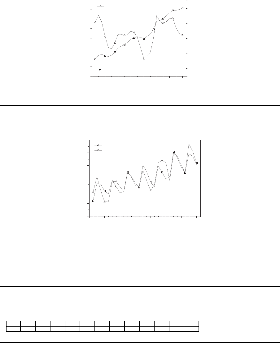
Beobachtungswerte und Prognose
100
200
300
400
500
600
700
Bedarfsmenge
0 4 8 12 16 20 24 28
Zeit
t
Beobachtung
Prognose
9 Ausgew¨ahlte Probleme
9.1 Bestimmung der Gl¨attungsparameter
Bestimmung der Gl¨attungsparameter
Beispiel
t 1 2 3 4 5 6 7 8 9 10 11 12
y
t
60 55 64 51 69 66 83 90 76 95 72 88
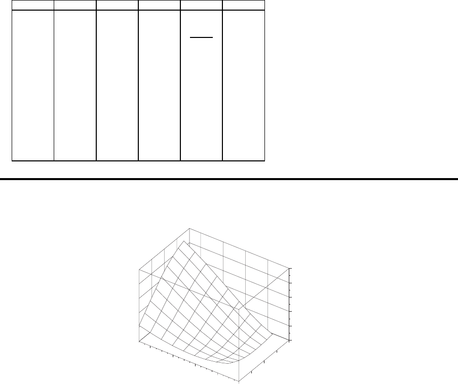
Mittlere quadrierte Fehler
26
β \ α 0.10 0.15 0.20 0.25 0.30
0.0050 112.44 106.87 103.92 102.76 102.88
0.0075 112.35 106.80 103.87 102.75 102.90
0.01 112.26 106.72 103.82 102.73 102.92
0.05 110.94 105.69 103.28 102.75 103.46
0.10 109.51 104.77 103.10 103.32 104.72
0.15 108.33 104.23 103.39 104.41 106.48
0.20 107.37 104.04 104.09 105.92 108.64
0.25 106.63 104.16 105.15 107.79 111.10
0.30 106.09 104.56 106.52 109.94 113.80
0.35 105.73 105.22 108.15 112.31 116.64
0.40 105.55 106.11 110.01 114.87 119.58
0.45 105.53 107.20 112.06 117.55 122.56
.
.
.
.
.
.
.
.
.
.
.
.
.
.
.
.
.
.
0.85 110.11 121.06 131.94 139.54 144.01
0.90 111.15 123.21 134.52 142.00 146.11
Mittlere quadrierte Fehler
0.2
0.4
0.6
0.8
0.10
0.15
0.20
0.25
0.30
100
110
120
130
140
150
α
β
mittlerer quadrierter
Prognosefehler
27