28 Stochastische Losgr¨oßenplanung
28.1 Einf¨uhrung
Strategien
• Dynamic uncertainty strategy: Produktionstermine und Produktionsmengen so sp¨at wie m¨oglich
festlegen
• Static-dynamic uncertainty strategy: Produktionstermine ex ante festlegen, Produktions mengen
reaktiv festlegen
• Static uncertainty strategy: Produktionstermine und Produktionsmengen ex ante festlegen
28.2 Fixe Produktionsmengen und -termine und
Static Uncertainty: Annahmen
• Dynamische Nachfrage
Periode t 25/2017 26/2017 . . . 35/2017
µ
t
. . . . . . . . . . . .
σ
t
. . . . . . . . . . . .
• Unbegrenzte Kapazit¨at
• Ex-ante Bestimmung eines Produktionsplans (Termine und Mengen)
• entweder: Fehlbestandskosten
• oder: Zyklusbezoge ne r β-Servicegrad β
⋆
c
Servicegrade
unter dynamischen Bedingungen
• α-Servicegrad
α
p
= P {Periodennachfragemenge
≤ phys ischer Bestand zu Beginn einer Periode}
α
c
= P{Nachfragemenge in der Wiederbeschaffung szeit
≤ physischer Bestand zu Beginn der Wiederbeschaffungsze it}
• β-Servicegrad
β = 1 −
E {Fehlmenge pro Periode}
E {Periodennachfragemenge}
= 1 −
E{B}
E{D}
113

Servicegrade
unter dynamischen Bedingungen
• β
c
-Servicegrad
β
c
= 1 −
E {Fehlmenge pro Produktionsz yklus}
E {Nachfrage pro Produktionszyklus}
First-order loss function f¨ur standard-no rmalverteilte Nachfrage:
Φ
1
(v)=
∞
R
v
(x − v) · φ(x) · dx
=
∞
R
v
x · φ(x) · dx − v ·
∞
R
v
φ(x) · dx
= φ (v) − v · {1 − Φ (v)}
= φ(v) − v ·Φ
0
(v)
(1)
mit
Φ
0
(v) =
∞
R
v
φ(x) · dx = 1 −Φ(v)
(2)
Ist die Variable Y mit µ
Y
und σ
Y
normalverteilt, dann gilt:
G
1
(s) = σ
Y
· Φ
1
(v)
(3)
mit v =
s − µ
Y
σ
Y
Static Uncertainty: Modell mit Fehlbestandskosten
Fehlbestandskosten
Model SSIULSP
q
π
Minimize E{C} =
T
X
t=1
s · γ
t
+ h ·E{I
p
t
} + π · E{I
f
t
}
subject to
Q
(t−1)
≤ Q
(t)
t = 1, 2, . . . , T
Q
(t)
− Q
(t−1)
≤ M · γ
t
t = 1, 2, . . . , T
γ
t
∈ {0, 1} t = 1, 2, . . . , T
Q
(t)
≥ 0 t = 1, 2, . . . , T
Static Uncertainty
π Fehlbestandskostensatz
I
p
t
Lagerbestand =
h
Q
(t)
− Y
(t)
i
+
I
f
t
Fehlbestand =
h
Y
(t)
− Q
(t)
i
+
114
Static Uncertainty
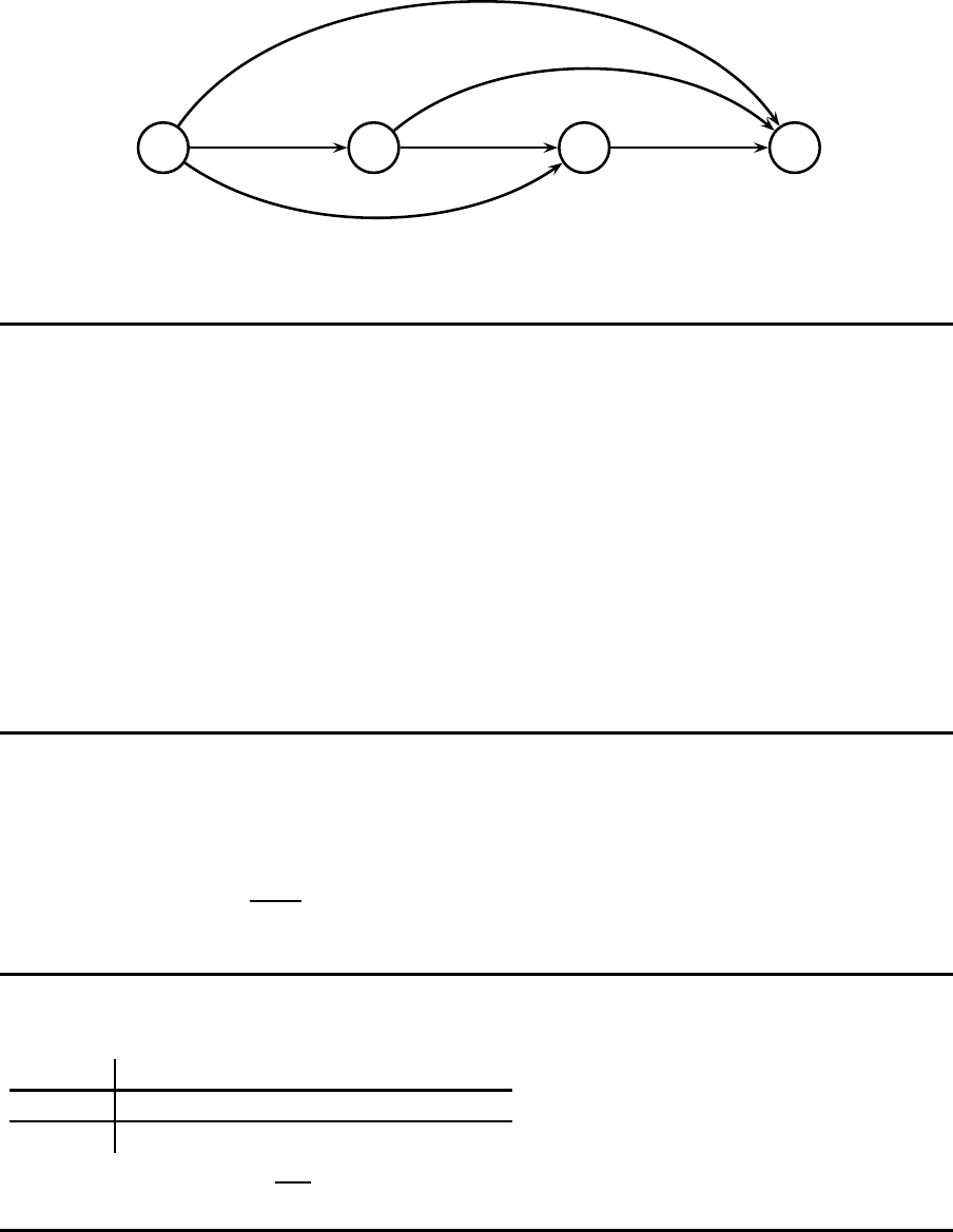
K¨urz este-Wege-Modell
1 2 3 4
E{C
12
} E{C
23
} E{C
34
}
E{C
24
}
E{C
14
}
E{C
13
}
Static Uncertainty
K¨urz este-Wege-Modell: Kosten eines Pfeils
E{C(Q
(ij)
} =
= s +
j−1
X
t=i
h ·
Q
(ij)
Z
0
(Q
(ij)
− y) · f
Y
(t)
· dy + π ·
∞
Z
Q
(ij)
(y −Q
(ij)
) · f
Y
(t)
·dy
= s +
j−1
X
t=i
h
h ·
Q
(ij)
opt
− E{Y
(t)
} + G
1
Y
(t)
(Q
(ij)
opt
)
+ π ·G
1
Y
(t)
(Q
(ij)
opt
)
i
Static Uncertainty
K¨urz este-Wege-Modell: Optimale Losgr¨oße
j−1
X
t=i
F
Y
(t)
(Q
(ij)
opt
) = (j − i) ·
π
h + π
Static Uncertainty
Beispiel I: Daten
t
1 2 3 4 5 6
E{D
t
} 200 50 100 300 150 300
σ
D
t
60 15 30 90 45 90
s = 1000, h = 1, π = 18,
π
h+π
= 0.9474.
115
Static Uncertainty
Beispiel II
i\j
2 3 4 5 6 7
1 0.9474 1.8947 2.8421 3.7895 4.7368 5.6842
2 – 0.9474 1.8947 2.8421 3.7895 4.7368
3
– – 0.9474 1.8947 2.8421 3.7895
4 – – – 0.9474 1.8947 2.8421
5 – – – – 0.9474 1.8947
6
– – – – – 0.9474
Static Uncertainty
Beispiel III: Optimale kumulierte Produktionsmengen
i\j
2 3 4 5 6 7
1 297.31 332.41 420.02 741.27 884.63 1173.26
2 – 350.21 436.62 763.76 903.53 1196.36
3
– – 461.42 791.95 926.22 1222.15
4 – – – 833.54 955.11 1252.24
5 – – – – 997.50 1289.83
6
– – – – – 1345.52
Static Uncertainty
Beispiel IV: Kosten
i\j
2 3 4 5 6 7
1 1122.47 1270.19 1566.16 2771.04 3522.11 5274.31
2 – 1126.24 1338.34 2219.01 2828.35 4289.80
3 – – 1140.31 1691.97 2163.98 3330.92
4
– – – 1231.16 1574.19 2444.34
5 – – – – 1248.74 1824.35
6
– – – – – 1309.23
116