Teil VI
Grundlagen der Bestandsmanagements
19.1 Modellierung von Supply Chains
Grundbegriffe I
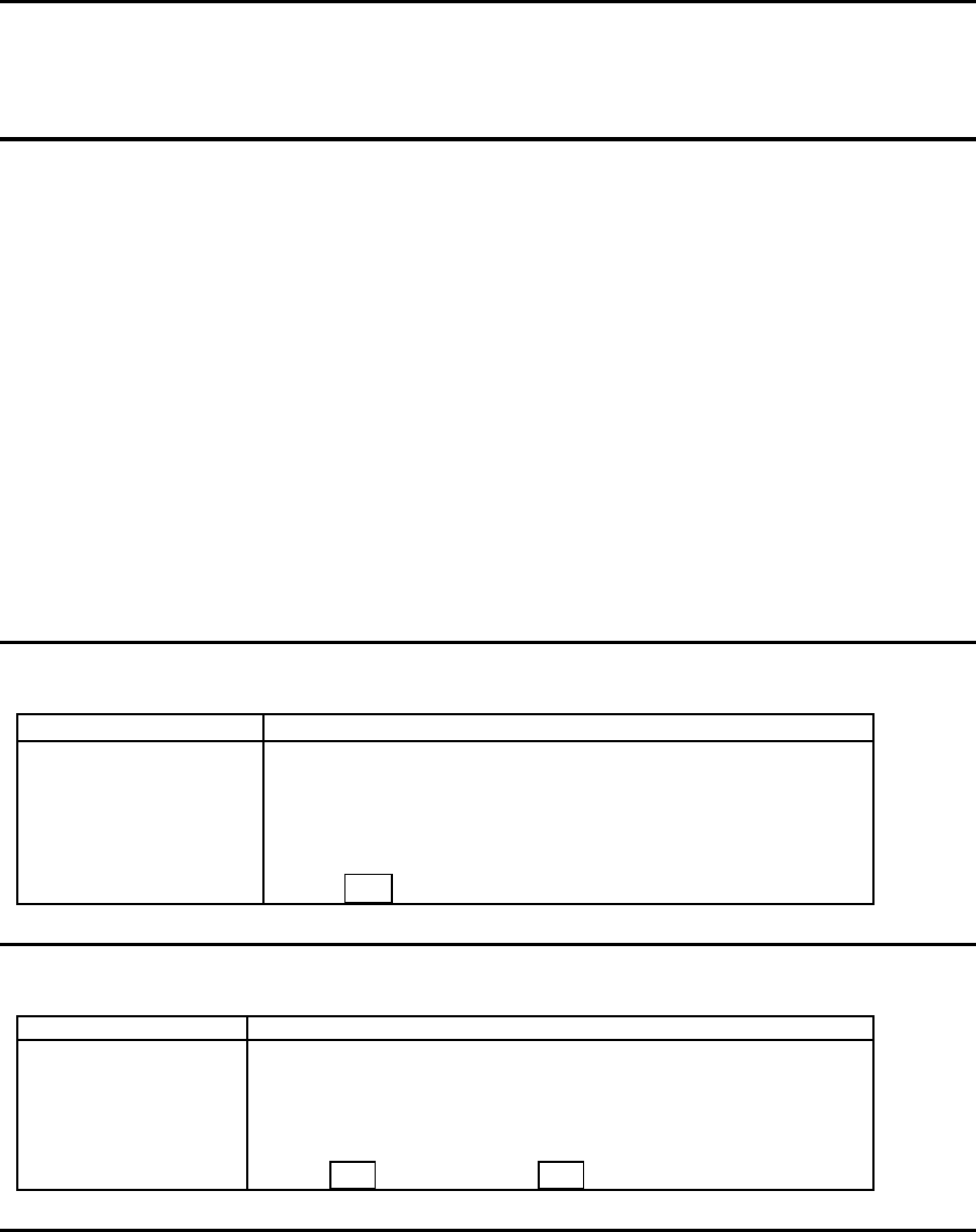
• Physischer Bestand: I
p
t
• Bestellbestand: I
o
t
• Fehlbestand: I
f
t
• Fehlmenge: F
• Nettobestand: I
n
t
I
n
t
= I
p
t
− I
f
t
• Disponibler Bestand: I
d
t
I
d
t
= I
n
t
+ I
o
t
Grundbegriffe II
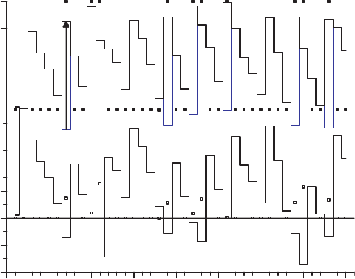
Periode t 0 1 2 3 4 5 6 7 8
Nachfrage d
t
– 59 54 50 83 44 57 46 54
Physische r Bestand I
p
t
248 189 135 85 2 0 0 255 201
Bestellbestand I
o
t
– 0 400 400 400 400 400 0 0
Fehlbe stand I
f
t
– 0 0 0 0 42 99 0 0
Nettobestand I
n
t
248 189 135 85 2 -42 -99 255 201
Disponibler Bestand I
d
t
248 189 535 485 402 358 301 255 201
Grundbegriffe II
Periode t 0 1 2 3 4 5 6 7 8
Nachfrage d
t
– 59 54 50 83 44 57 46 54
Physischer Bestand I
p
t
248 189 135 85 2 0 0 55 1
Bestellbestand I
o
t
– 0 200 200 200 400 400 200 200
Fehlbestand I
f
t
– 0 0 0 0 42 99 0 0
Nettobestand I
n
t
248 189 135 85 2 -42 -99 55 1
Disponibler Bestand I
d
t
248 189 335 285 202 358 301 255 201
73
Grundbegriffe IV
-200
-100
0
100
200
300
400
500
600
700
800
M
e
n
g
e
0 5 10 15 20 25 30 35 40
Zeit
Nettobestand
disponibler
Bestand
74
20 Produktbezogene Leistungskriterien eines Lagers
20.1 α-Servicegrad
α-Servicegrad
α
Per
= P {Periodennachfragemenge
≤ physischer Bestand zu Beginn einer Periode}
α
Zyk
= P {Nachfragemenge in der Wiederbeschaffungszeit
≤ physischer Bestand zu Beginn
der Wiederbeschaffungszeit}
Beispiel
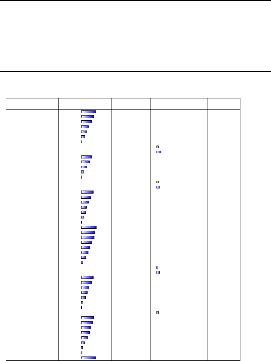
Periode Nachfrage
Bestand Bestellung oder Fehlbestand Fehlmenge
(physisch) Wareneingang (Periodenende) (pro Zyklus)
1 50 350 – –
2 58 292 – –
3 44 248 – –
4 59 189 ⇒ – –
5 54 135 – –
6 50 85 – –
7 83 2 – –
8 44 – 42 –
9 57 – ⇐ 99 99
10 46 255 – –
11 54 201 ⇒ – –
12 74 127 – –
13 64 63 – –
14 46 17 – –
15 57 – 40 –
16 38 – ⇐ 78 78
17 34 288 – –
18 58 230 ⇒ – –
19 53 177 – –
20 54 123 – –
21 18 105 – –
22 44 61 – –
23 54 7 ⇐ 0 0
24 46 361 – –
25 38 323 – –
26 14 309 – –
27 55 254 – –
28 56 198 ⇒ – –
29 36 162 – –
30 57 105 – –
31 71 34 – –
32 60 – 26 –
33 45 – ⇐ 71 71
34 42 287 – –
35 35 252 – –
36 67 185 ⇒ – –
37 40 145 – –
38 45 100 – –
39 59 41 – –
40 33 8 – –
41 50 – ⇐ 42 42
42 67 291 – –
43 16 275 – –
44 46 229 ⇒ – –
45 32 197 – –
46 40 157 – –
47 77 80 – –
48 51 29 – –
49 28 1 ⇐ 0 0
50 60 341 – –
75
20.2 β-Servicegrad
β-Servicegrad
β = 1 −
E {Fehlmenge pro Periode }
E {Periodennachfragemenge}
• Nachfrage 49.18
• Fehlmenge 5.8
• β-Servicegrad = 88.21
20.3 γ-Servicegrad
γ-Servicegrad
γ = 1 −
E {Fehlbestand pro Periode}
E {Periodennachfragemenge}
• Nachfrage 49.18
• Fehlbe stand 7.96
• β-Servicegrad = 83.81
21 Die Kennziffer ’Bestandsreichweite’
Bestandsreichweite
• Saisonaler Bestand
• Losgr¨oßenbestand
• Transportlosgr¨oßenbestand
• Transitbestand
• Kommissionierbestand
• Sicherheitsbestand
SB = v
opt
·σ
Y
76
22 Exkurs: Wahrscheinlichkeitsverteilungen
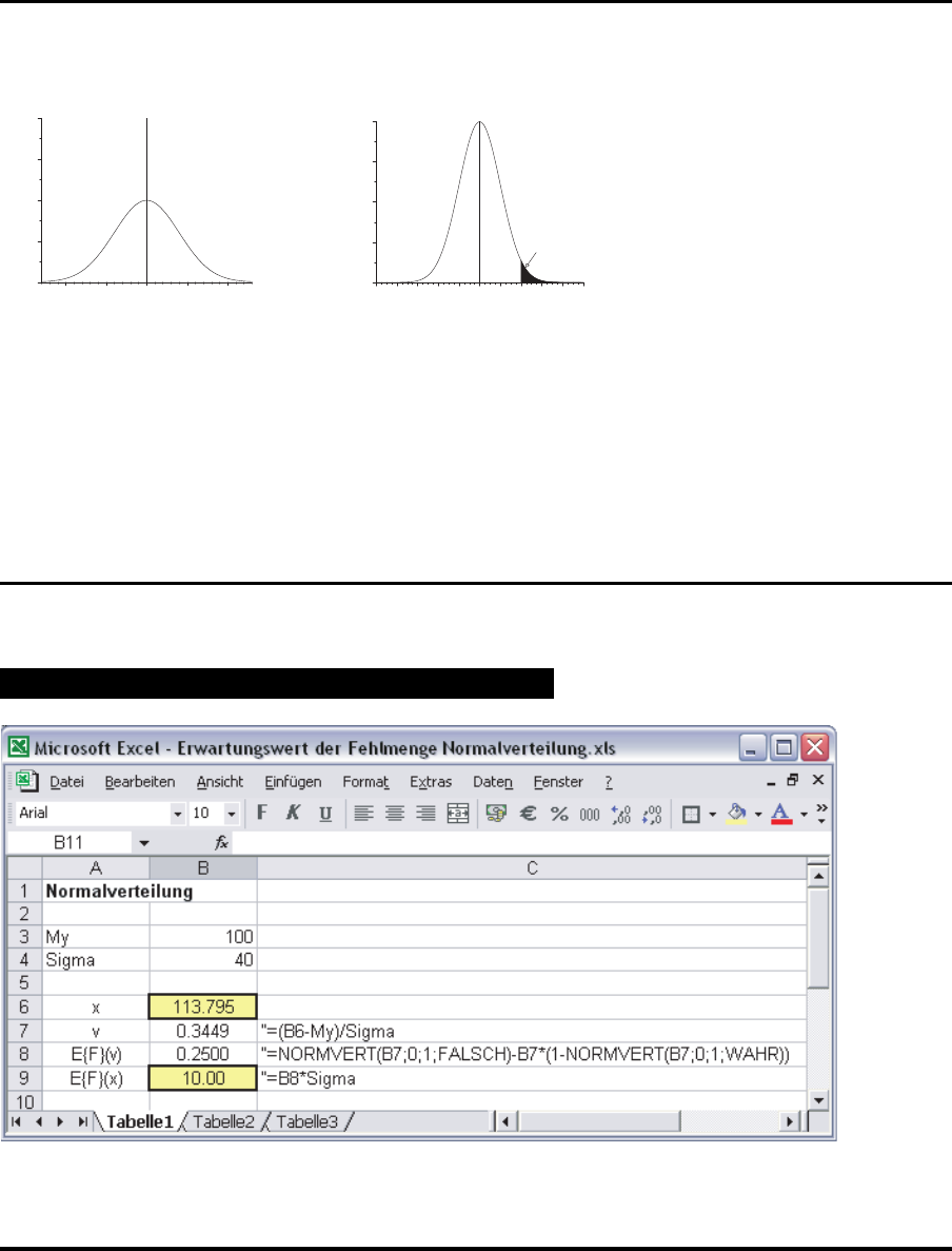
22.1 Normalverteilung
Normalverteilung
N(µ
Y
, σ
Y
) N(µ
X
= 0, σ
X
= 1)
0.0
0.1
0.2
0.3
0.4
0 5 10 15 20
y
f
Y
(y)
⇒
0.0
0.1
0.2
0.3
0.4
-5 -4 -3 -2 -1 0 1 2 3 4 5
x
v
φ(x)
P {x ≥ v}
Φ
0
(v) =
∞
Z
v
φ(x) · dx = 1 − Φ(v)
Φ
1
(v) =
∞
Z
v
(x − v) · φ(x) · dx = φ(v) −v · Φ
0
(v)
Normalverteilung II: Excel
NORMVERT(x;0;1;FALSCH)-x*(1-NORMVERT(x;0;1;WAHR))
22.2 Gamma-Verteilung
77
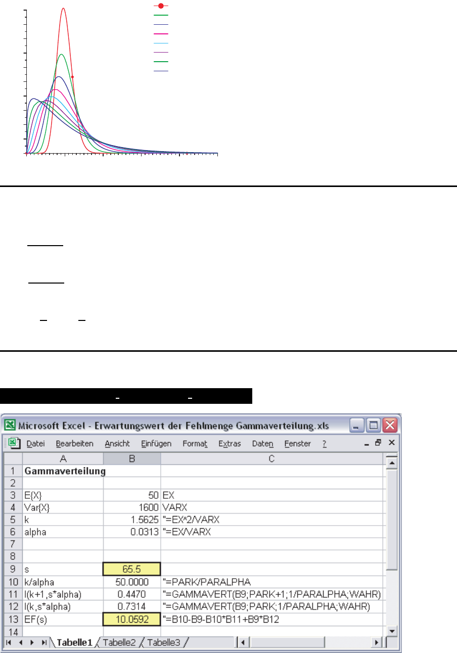
Gamma-Verteilung I
0.00
0.02
0.04
0.06
0.08
0.10
0.12
0.14
0.16
0.18
0.20
Dichtefunktion f(x)
0 10 20 30 40 50
Bearbeitungszeit
E{X}=10;V{X}=4
E{X}=10; V{X}=9
E{X}=10;V{X}=16
E{X}=10;V{X}=25
E{X}=10;V{X}=36
E{X}=10;V{X}=49
E{X}=10;V{X}=64
E{X}=10;V{X}=81
Gamma-Verteilung II
k
Y
=
E {Y }
2
Var {Y }
α
Y
=
E {Y }
Var {Y }
G
1
(s) =
k
α
− s −
k
α
·I [k + 1, s · α] + s · I [k, s ·α]
Gamma-Verteilung III: Excel
GAMMAVERT(x;Parameter k;1/Parameter alpha;WAHR)
78
23 Nachfragemenge im Risikozeitraum
Nachfragemenge im Risikozei traum
f
D
(d)
F
D
(d) = P {D ≤ d}
P {D = d, d = d
min
, ..., d
max
}
23.1 Deterministische Wiederbeschaffungszeiten
Deterministische Wiederbeschaffungszeiten
Normalverteilung
D
σ
D
µ
Y
= µ
D
·ℓ
σ
Y
= σ
D
·
√
ℓ
Deterministische Wiederbeschaffungszeiten
Gamma-Verteilung
D
α
D
k
D
α
Y
= α
D
k
Y
= k
D
· ℓ
79
Deterministische Wiederbeschaffungszeiten
Diskrete empirische Verteilung
P
Y
1
= y
k
= P {D = y
k
}
P
Y
ℓ
= y
k
=
X
x
i
+d
j
=y
k
P
Y
ℓ−1
= x
i
, D = d
j
ℓ ≥ 2
Deterministische Wiederbeschaffungszeiten
ℓ = 1 : 0 ≤ y
k
≤ 2
P
Y
1
= 0
= 0.1
P
Y
1
= 1
= 0.4
P
Y
1
= 2
= 0.5
Deterministische Wiederbeschaffungszeiten
ℓ = 2 : 0 ≤ y
k
≤ 2 + 2 = 4
P
Y
2
= 0
= P
Y
1
= 0
·P {D = 0}
= 0.1 · 0.1 = 0.01
P
Y
2
= 1
= P
Y
1
= 0
·P {D = 1}
+ P
Y
1
= 1
·P {D = 0}
= 0.1 · 0.4 + 0.4 · 0.1 = 0.08
P
Y
2
= 2
= P
Y
1
= 0
·P {D = 2}
+ P
Y
1
= 1
·P {D = 1}
+ P
Y
1
= 2
·P {D = 0}
= 0.1 · 0.5 + 0.4 · 0.4 + 0.5 · 0.1 = 0.26
P
Y
2
= 3
= P
Y
1
= 1
·P {D = 2}
+ P
Y
1
= 2
·P {D = 1}
= 0.4 · 0.5 + 0.5 · 0.4 = 0.40
P
Y
2
= 4
= P
Y
1
= 2
·P {D = 2}
= 0.5 · 0.5 = 0.25
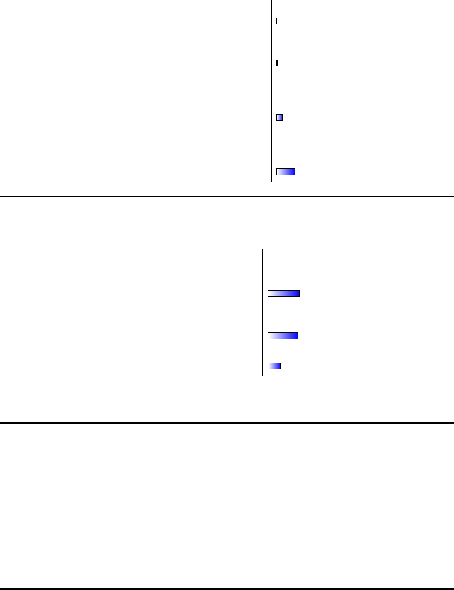
Deterministische Wiederbeschaffungszeiten
ℓ = 3 : 0 ≤ y
k
≤ 4 + 2 = 6 (I)
80
P
Y
3
= 0
= P
Y
2
= 0
· P {D = 0}
= 0.01 · 0.1 = 0.001
P
Y
3
= 1
= P
Y
2
= 0
· P {D = 1}
+ P
Y
2
= 1
· P {D = 0}
= 0.01 · 0.4 + 0.08 · 0.1 = 0.012
P
Y
3
= 2
= P
Y
2
= 0
· P {D = 2}
+ P
Y
2
= 1
· P {D = 1}
+ P
Y
2
= 2
· P {D = 0}
= 0.01 · 0.5 + 0.08 · 0.4 + 0.26 · 0.1 = 0.063
P
Y
3
= 3
= P
Y
2
= 1
· P {D = 2}
+ P
Y
2
= 2
· P {D = 1}
+ P
Y
2
= 3
· P {D = 0}
= 0.08 · 0.5 + 0.26 · 0.4 + 0.4 · 0.1 = 0.184
Deterministische Wiederbeschaffungszeiten
ℓ = 3 : 0 ≤ y
k
≤ 4 + 2 = 6 (II)
P
Y
3
= 4
= P
Y
2
= 2
·P {D = 2}
+ P
Y
2
= 3
·P {D = 1}
+ P
Y
2
= 4
·P {D = 0}
= 0.26 · 0.5 + 0.4 · 0.4 + 0.25 · 0.1 = 0.315
P
Y
3
= 5
= P
Y
2
= 3
·P {D = 2}
+ P
Y
2
= 4
·P {D = 1}
= 0.4 · 0.5 + 0.25 · 0.4 = 0.300
P
Y
3
= 6
= P
Y
2
= 4
·P {D = 2}
= 0.25 · 0.5 = 0.125
23.2 Stochastische Wiederbeschaffungszeiten
Stochasti sche Wiede rbeschaffungszeiten I
E {Y } = E {L}· E {D}
Var {Y } = E {L} · Var {D} + Var {L} · E {D}
2
f
Y
(y) =
ℓ
max
X
ℓ=ℓ
min
f
Y
(y |L = ℓ) · P {L = ℓ}
Stochasti sche Wiede rbeschaffungszeiten II
F
Y
(y) =
ℓ
max
X
ℓ=ℓ
min
y
Z
0
f
Y
(x |L = ℓ) · dx · P {L = ℓ}
81
P {Y ≤ y} =
ℓ
max
X
ℓ=ℓ
min
P {Y ≤ y |L = ℓ } · P {L = ℓ}
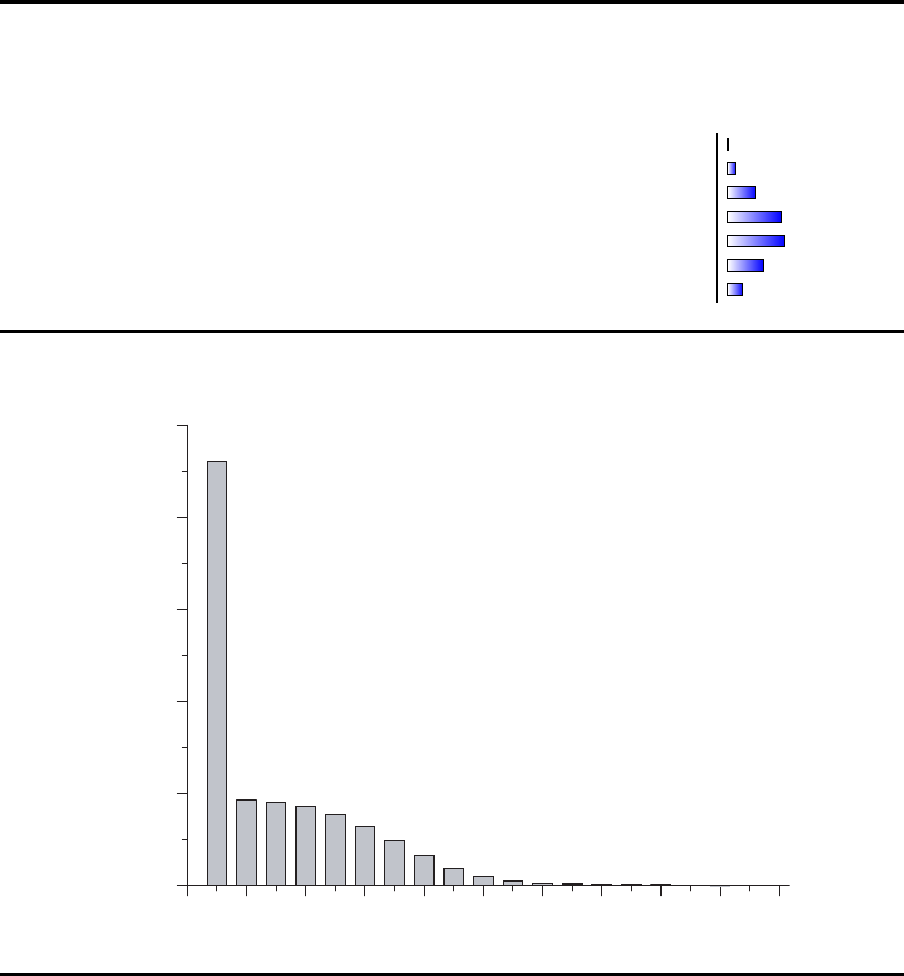
Stochasti sche Wiede rbeschaffungszeiten III
P {L = 2} = 0.4 und P {L = 3} = 0.6
P {Y = 0} = P
Y
2
= 0
· 0.4 + P
Y
3
= 0
· 0.6 = 0.004 + 0.0006 = 0.0046
P {Y = 1} = P
Y
2
= 1
· 0.4 + P
Y
3
= 1
· 0.6 = 0.032 + 0.0072 = 0.0392
P {Y = 2} = P
Y
2
= 2
· 0.4 + P
Y
3
= 2
· 0.6 = 0.104 + 0.0378 = 0.1418
P {Y = 3} = P
Y
2
= 3
· 0.4 + P
Y
3
= 3
· 0.6 = 0.160 + 0.1104 = 0.2704
P {Y = 4} = P
Y
2
= 4
· 0.4 + P
Y
3
= 4
· 0.6 = 0.100 + 0.1890 = 0.2890
P {Y = 5} = P
Y
2
= 5
· 0.4 + P
Y
3
= 5
· 0.6 = 0 + 0.1800 = 0.1800
P {Y = 6} = P
Y
2
= 6
· 0.4 + P
Y
3
= 6
· 0.6 = 0 + 0.0750 = 0.0750
Stochasti sche Wiede rbeschaffungszeiten IV
0.0
0.1
0.2
0.3
0.4
0.5
P
{
L=
}
0 2 4 6 8 10 12 14 16 18 20
`
`
Stochasti sche Wiede rbeschaffungszeiten V
82
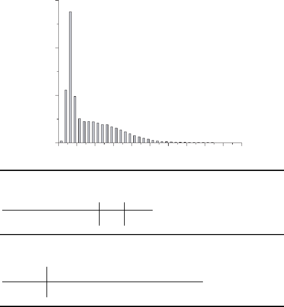
0.0
0.1
0.2
0.3
P
{
Y
=
y
}
0 200 400 600 800 1000 1200 1400 1600 1800 2000
yy
Stochasti sche Wiede rbeschaffungszeiten VI
Deterministische WBZ
Wiederbeschaffungszeit ℓ 5 10
Bestellpunkt 521.1 1036.78
Durchschnittlicher Lagerbestand 426.74 442.88
Stochasti sche Wiede rbeschaffungszeiten VI
Stochastische WBZ
P {L = 5} – 0.2 0.4 0.6 0.8 1.0
P {L = 10} 1.0 0.8 0.6 0.4 0.2 –
Bestellpunkt 1036.78 1016.23 986.43 935.54 804.77 521.10
Lagerbestand 442.88 522.54 593.08 642.89 614.47 426.74
Stochasti sche Wiede rbeschaffungszeiten VIII
Stochastische WBZ
83
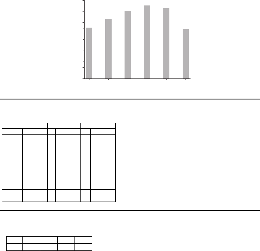
0
100
200
300
400
500
600
700
L
a
g
e
r
b
e
s
t
a
n
d
1.0|0.0 0.8|0.2 0.6|0.4 0.4|0.6 0.2|0.8 0.0|1.0
P{L=10}|P{L=5}
L=10 L=5
stochastische Wiederbeschaffungszeit
Stochasti sche Wiede rbeschaffungszeiten VIII
Fall 2 Fall 3 Fall 4
ℓ P {L = ℓ} ℓ P {L = ℓ} ℓ P {L = ℓ}
3 0.3 2 0.2548 2 0.35
4 0.4 3 0.2162 3 0.24
5 0.3 4 0.1776 4 0.13
5 0.1390 5 0.05
6 0.1005 6 0.05
7 0.0619 7 0.05
8 0.0500 8 0.05
9 0.05
10 0.02
11 0.01
E{L} 4 4 4
Var{L} 0.60 3.13 5.60
Stochasti sche Wiede rbeschaffungszeiten VII
Fall 1 2 3 4
β 86.6 84.4 81.1 79.9
84