21
41 Dynamische stochastische Losgr¨oßenplanung
K¨urzeste-Wege-Mo dell
E{C(Q
(ij)
} =
s +
j−1
X
t=i
h ·
Q
(ij)
Z
0
(Q
(ij)
−y) · f
Y
(t)
· dy + π ·
∞
Z
Q
(ij)
(y − Q
(ij)
) · f
Y
(t)
· dy
Diese Funktion hat die Str uktur der Zielfunktion des Newsvendor-Problems. Der optimale
Wert von Q
(ij)
kann mit Hilfe der folgenden Optimalit¨atsbedingung bestimmt werden:
j−1
X
t=i
F
Y
(t)
(Q
(ij)
opt
) = (j − i) ·
π
h + π
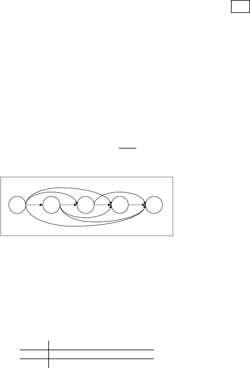
1 2 3 4 T+1
E{C(Q
(14)
opt
)}
Figure 2: K¨urzeste-Wege-Graph
E{C(Q
(ij)
opt
)} =
s +
j−1
X
t=i
h
h ·
Q
(ij)
opt
− E{Y
(t)
} + G
1
Y
(t)
(Q
(ij)
opt
)
+ π · G
1
Y
(t)
(Q
(ij)
opt
)
i
t 1 2 3 4 5 6
E{D
t
} 200 50 100 300 150 300
σ
D
t
60 15 30 90 45 90
261
i\j 2 3 4 5 6 7
1 0.9474 1.8947 2.8421 3.7895 4.7368 5.6842
2 – 0.9474 1.8947 2.8421 3.7895 4.7368
3 – – 0.9474 1.8947 2.8421 3.7895
4 – – – 0.9474 1.8947 2.8421
5 – – – – 0.9474 1.8947
6 – – – – – 0.9474
i\j 2 3 4 5 6 7
1 297.31 332.41 420.02 741.27 884.63 1173.26
2 – 350.21 436.62 763.76 903.53 1196.36
3 – – 461.42 791.95 926.22 1222.15
4 – – – 833.54 955.11 1252.24
5 – – – – 997.50 1289.83
6 – – – – – 1345.52
Table 7: Optimale kumulierte Produktionsmengen Q
(ij)
opt
i\j 2 3 4 5 6 7
1 1122.47 1270.19 1566.1 6 2771.04 352 2.11 5274.31
2 – 1126.24 1338.34 2219.01 2828.35 4289.80
3 – – 1140.31 1691.97 2163.9 8 3330.92
4 – – – 1231.16 1574.19 2444.34
5 – – – – 1248.74 1824.35
6 – – – – – 1309 .23
Table 8: Kosten
262