Modeling of the Time Axis
For the analysis of an inventory policy the modeling of the time axis is important in several respects. Not only does the length of the review period (review interval) matter, but also assumptions concerning the structure of the customer order arrivals must be made.
The review period is the length of the interval between two consecutive inventory reviews. In the literature, periodic and continuous review are discussed. With periodic review the inventory records are updated in regular intervals, say, at the end of each day or every two weeks. Depletions of the inventory which happen within a review period are only recognized at the next review instant with a more or less large delay. It is only then possible to react on an unusually great demand through the placement of a replenishment order. The additional stock-out risk that results from this delay must be absorbed through an increased safety inventory.
The same situation as with periodic review arises when the demand per customer order is greater than unity. If a customer purchases, say, ten units of a product, then the inventory records are only updated after the removal of the complete demand. Even if immediately after that event a replenishment order is released, it is possible that the inventory may have fallen far below the minimum level used as the criterion for the placement of a replenishment order. This may be observed even in a super market when a customer buys three jars of yoghurt of the same flavor. Once he has removed the jars from the shelf, he walks around the market to select further products. By the time he arrives at the cash counter where the product removal is registered by a scanner, the inventory may have already fallen below the reorder point. The additional stock-out risk which results from this delay must also be taken into account in the determination of the control parameters of some inventory policies.
With continuous review the situation is different. Here, it is assumed that precise data on the inventory status are available at any point in time and that a replenishment order can be launched and is handled by the supplier without delay. This will only be the case if, besides a continuous time axis, the customer orders are unit-sized. In many inventory models assuming continuous review, the additional assumption is made that the length of the replenishment lead time is deterministic. This means that the amount ordered from a supplier at time $t$ will arrive exactly at time $t+\ell$. Thereby, it is usually neglected that a replenishment order triggers an order handling process in the supplier's logistics system which may involve several phases, such as material handling, packaging, delivery by a logistic service provider, etc. In many companies delivery trucks start their tours in the morning independently of the exact arrival times of the customer orders in the preceding day. Even if the replenishment order has been launched and transmitted to the supplier via internet, the order will nevertheless arrive at discrete points in time, for example at the beginning of the next day. Thus, even with continuous review, one often observes a discretization of the time axis. Depending on the precise time of the order release, this behavior of the supplier's logistics system will lead to non-deterministic lead times.
Another aspect that must be taken into account refers to the type of the time axis of customer arrivals. Many inventory models assume customers arriving on a continuous time axis. For example, in inventory models for spare parts it is assumed that the intervals between consecutive arrivals of unit-sized demands follow an exponential distribution which is equivalent to Poisson arrivals of customers on a continuous time axis.
It is also often supposed that the demands result from orders which arrive on a continuous time axis with interarrival time $A$, where each order has a random order size $D^a$ ("compound demand"). The demand process over time is then characterized by the pair of random variables $(A_n,D_n^a)$ $(n=1,2,\ldots)$.
The concrete form of the demand process depends on the interarrival times of the orders and on the order sizes.
Additional information are available in the book.
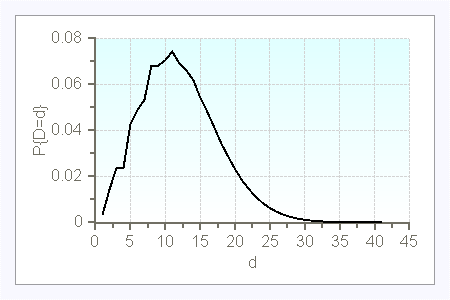
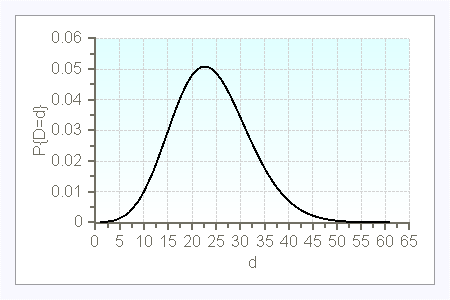
In the case of compound Poisson demand, the interarrival times $A$ follow an exponential distribution with parameter $\lambda$, and the order size $D^a$ is a nonnegative - usually discrete - random variable. If $D^a$ is deterministic equal to 1, then the demand process is a simple Poisson process. The probability distribution of the demand per time period can be computed with the following recursion for $t\geq 0$:
$P\{D=0\}=e^{-\lambda\cdot t\cdot (1-P\{D^a=0\})$
and
$P\{D=d\}=\frac{\lambda\cdot t}{d} \cdot\displaystyle{ \sum_{j=0}^{d-1}} (d-j)\cdot P\{D^a=d-j\}\cdot P\{D=j\} \qquad d=1,2,\ldots$
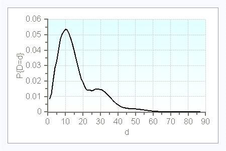
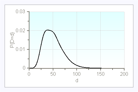
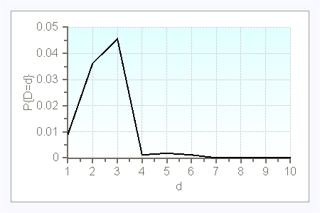
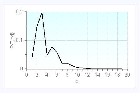
Here are a few examples of compound Poisson demands (with $t=1$):
$d$ |
$P\{D^a=d\}$ |
1 |
0.25 |
2 |
0.20 |
3 |
0.30 |
4 |
0.20 |
20 |
0.05 |
$\lambda=5$
$\lambda=15$
$d$ |
$P\{D^a=d\}$ |
1 |
0.10 |
2 |
0.40 |
3 |
0.50 |
$\lambda=0.1$
$\lambda=1$
$\lambda=5$
$\lambda=10$
Additional information, e.g. on compound renewal demands, are available in the here.