|
Inventory management: (s,q) inventory policy with normal-distributed period demand
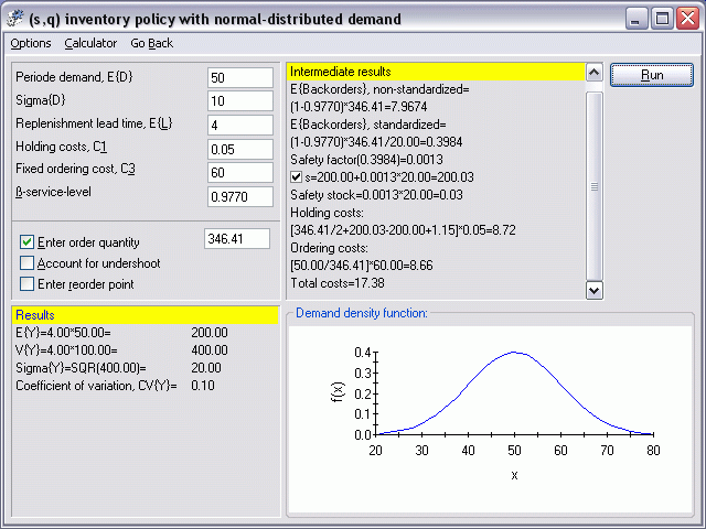
A (s,q) inventory policy for a product with normal-distributed demand per
period and a fixed lead time is computed. In the standard version, continuous
review is assumed. In this case, an iterative algorithm for finding the optimal
values of s and q is applied. Alternatively, reviewing the inventory position
at the end of each period (e.g. a day) while maintaining a fixed-quantity q
[opposite to the (s,S) policy] is assumed. In this case the expectation and
variance of the undershoot variable is computed and integrated into the computation
of s.
Symbols:
| E{D} |
expected demand per period |
| E{L} |
lead time |
| E{Y} |
expected demand during lead time |
| V{Y} |
variance of the demand during lead time |
| E{Y*} |
expected value of the sum of the demand during lead time and the undershoot |
| V{Y*} |
variance of the sum of the demand during lead time and the undershoot |
| E{U} |
expected undershoot |
| V{U} |
variance of the undershoot |
| P{.} |
probability |
| s |
reorder point |
| q |
order size |
Assumptions:
- normal-distributed demand
- ß-service level
- backorders, no lost sales
After computation of the optimal values of s and q these values are transfered
to the simulation module.
Literature:
- Tempelmeier (2006)
|