Supply Network Planning (single stage)
This module solves basic models in the field of aggregate production planning.
This type of problem is supported by commercially available Advanced Planning Systems and
is called Supply Network Planning. The following decision variables are considered:
- Inventory build-up
- Overtime
- Purchasing from an external supplier
The objective is to minimize the sum of all related costs under
the constraint that all demands must be fullfilled in time.
This module generates and solves a linear optimization model for different planning
situations. At most two factories
and one
supplier may be considered. A maximum 3 products
and 24 periods may be considered. The resulting
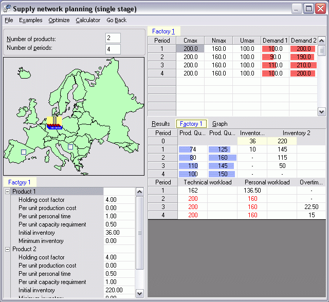
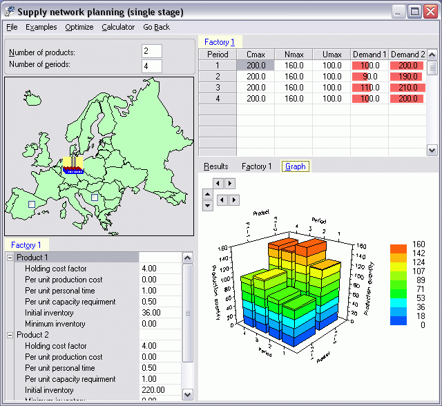
linear optimization models comprises up to 700 variables. The user interface
is a follows:


In this module only single-stage systems are considered. I.e. all factories and the supplier are producing end products.
The situation where components are produced in one factory and end products
are produced in the second factory is not considered her. For this type of problem
see the module "Supply Network Planning (two-stages)".
Each factory fills its own demands for the products. Through the
introduction of transport relations a system-wide optimization is possible.
In each factory maximum total inventory
capacities as well as product-specific minimum
inventory levels can be considered.
You can solve all the models with SAP's module SNP
which is part of the Advanced Planner and Optimizer.
In what follows several applications of the module are discussed.
You may wish to consider these problems step-by-step and save the data entered
in a file for later re-use.
1. A single factory
The easiest type of problem is to consider a single
factory. This is the typical aggregate production planning problem discussed in many production
and operations management textbooks. The objective is the sum of inventory costs
and overtime costs.
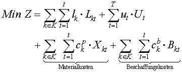
The linear optimizatin model read as follows:

subject to


Symbols:
| k |
index of products |
| t |
index of periods |
| a(k) |
human capacity absorption factor of product k |
| b(k) |
technical capacity absorption factor of product k |
| l(k) |
inventory holding costs |
| u(t) |
overtime costs |
| C(t)max |
maximum technical capacity |
| U(t)max |
maximum overtime |
| N(t)max |
normal human capacity |
| L(kt) |
inventory of product k at the end of period t |
| U(t) |
overtime hours used |
| X(kt) |
production quantity of product k in in period t |
This basic model can be extended through the inclusion of inventory
constraints with respect to the maximum total inventory and the minimum product-specific inventory.
2.Two factories
Assume that we have two factories that can produce the same products.
Instead of using overtime in a certain period in factory 1 it might be economical
to use standard capacity in factory 2 and transport the products to factory
1. In this case, we must include the transportation costs into the objective
function. The quantity of product k transported in period t from factory 1 to
factory 2 is denoted F(12kt). The flow in the opposite direction is denoted
F(21kt). The introduction of a second location requires the use of an additional
idex s. The objective function reads as follows:

The inventory balance equations are given by

Additional symbols:
| f(ij) |
transportation costs per unit between factory i und
factory j |
| F(ijkt) |
transportion quantity from factory i to factory
j |
3. One factory and one supplier
Assume that an external supplier produces the same products as
factory 1. In this case in addition to the inventory and overtime costs the
objective function comprises the external purchasing costs and the variable
production costs.

The inventory balance equations are augmented by the purchased
quantity B(kt):

Additional symbols:
| c(bk) |
purchasing costs per unit |
| c(fk) |
variable production costs |
| B(kt) |
quantity purchased |
4. Two factories and one supplier
The situation results in the problem with
the maximum complexity.
Assumptions:
- linear objective function and constraints
- single-stage system, all locations produce the same
products dieselben Produkte
- maximum 3 products
- maximum 24 periods
- maximum two factory and one supply node (note that
this node may represent a single supplier for each product)
Tip: Following the
data input, a model generator generates the appropriate simplex tableau. The
LP is then solved with an internal solver. Note that commercially available
solvers (e.g. CPLEX or MOPS) are VERY MUCH FASTER.
Literature:
- Silver/Pyke/Peterson (1998)
|


