Time series analysis: ratio-to-moving-average procedure
The components of a time series are computed according to
ratio-to-moving-average method. The number of saesonal periods may be
4 or 12.
If a different number of seasonal periods is entered (e.g. 0), then the deseasonalization
procedure is skipped and only the trend line is computed by linear regression.
According to the ratio-to-moving-average method, the following steps are performed:
First, a centered moving-average is computed to find the smooth component TC
of the time series. Next, the seasonal factors SI are computed through the division
SI=Y/TC. Then, for each seasonal period the seasonal factor is estimated. Seasonal
factors are not standardized. Finally, the trend line is computed by linear
regression.
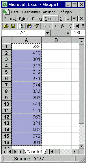
Data may be entered via the clipboard. In this case, a spreadsheet column must
me filled with the time series data and copied in to the clipboard.

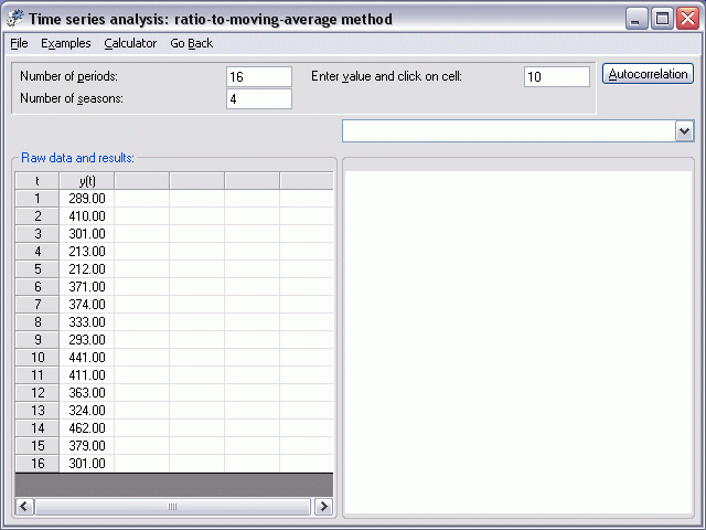
Then move the cursor into the first cell of the data entry table. With
(Shift - Left Mouse button) the contents of the clipboard is transfered.
The length of the times series should be recognized automatically.

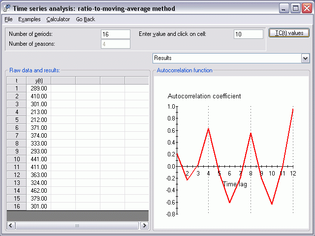
Before the decompostion starts, the autocorrelation
function is computed.

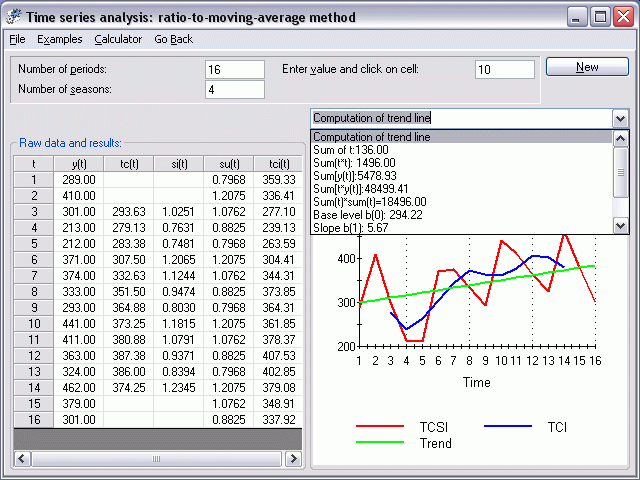
After the decomposition procedure is finished, you may wish to click on a cell
in the table to find out how the value displayed in the cell was computed.

Symbols:
| t |
index of time periods |
| tc(t) |
smooth component in period t |
| si(t) |
seasonal factor in period t |
| su(t) |
mean seasonal factor with respect to the season of
period t |
| tci(t) |
deseasonalized time series in period t |
| rho(j) |
autocorrelation coeffizient given a time lag of j
periods |
The seasonal factors and the parameters of trend line are automatically transfered
as initial values into the module "Procedure
of Winters ".
Literature:
- Tempelmeier (2005)
|


